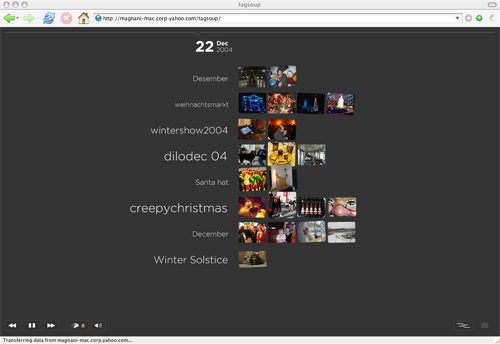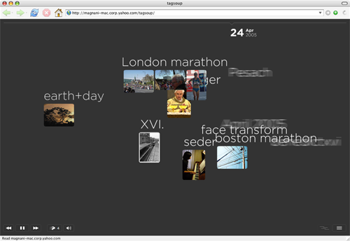
Figure 1: Screenshot of the river metaphor
.There is enormous and growing interest in the consumption of up-to-the-moment streams of newly-published content of various forms: news articles, posts on blogs or bulletin boards, and multimedia data such as images, songs, or movie clips. Users often consume such data on an as-generated basis, using mechanisms like atom and RSS to be notified when interesting content becomes available.
Social media applications like flickr.com, del.icio.us, rawsugar.com, technorati.com, stumbleupon.com, myweb.yahoo.com, and simpy.com, provide an opportunity for communities of users to build structure on top of base content using tags and annotations [14,4]. In Flickr for example, users may upload and share photos, and may place tags on their own or others' photos. It is possible then to browse through users, photos, tags, or more complex structures such as groups, themes, and clusters.
By watching the behavior of users in these social environments over time, we can explore the evolution of community focus. In this paper we study a browser-based application to visualize the evolution of ``interesting''1 tags in Flickr. In fact, our techniques apply broadly to materializing and visualizing sequences of ``interesting'' data points along a time series.
A satisfactory solution to this problem requires some means of addressing the problem of timescale: a time series may look very different at the scale of a single day than at the scale of a week, a month, or a year. Information at the daily level may be interesting and quirky, while information at the week or month level may show broader and more persistent patterns and shifts. Either may be of interest, depending on the user's intent. Our techniques will apply at any timescale, but coping with the complexity of this requirement without compromising efficiency requires us to develop some novel backend machinery.
These new temporal streams of information are generating data at a furious pace. It is certainly not possible to show all the information to the user, so the data must ``cooked'' in some way into a succinct summary tailored at the particular information needs of the user. In some cases, the user may seek data points that are particularly anomalous, while in other cases it may be data points that are highly persistent or that manifest a particular pattern. We focus on one particular notion of ``interesting'' data: the tags during a particular period of time that are most representative for that time period. That is, the tags that show a significantly increased likelihood of occurring inside the time period, compared to outside. We develop a novel visualization and a series of algorithms that allow the visualization to be produced efficiently over time.
The visualization itself has certain requirements: it must provide a view of temporal evolution, with a large amount of surface data easily visible at each timestep. It must allow the user to interact with the presentation in order to drill down into any particular result. It must remain ``situated,'' in the sense that the user must always be aware of the current point of time being presented, and it must provide random access into the time stream so that the user can reposition the current time as necessary. We present a family of evolving visualizations implemented in Actionscript/Flash MX that meet these requirements.
Our visualization makes use of two screen regions. First, a narrow timeline across the top of the page shows an interval representing the current time window. This interval slides forward as the animation progresses, and may be shifted by the user to provide random access into the overall time sequence. The remainder of the page shows interesting tags during the current time period. These tags enter and depart the page based on one of two metaphors: a `river' metaphor, in which tags flow in from the right and exit to the left and a `waterfall' metaphor, in which tag slots remain fixed but particular tags flow through the slots over time.
In order to drive the visualization, we develop backend algorithms to produce the necessary data. To generate the interesting tags for a particular time period, the scale of the data renders infeasible any scheme that must examine all the data before providing an answer. Thus, any real-time solution must provide a data structure that supports rapid generation of the relevant information. We consider techniques from database indexing, text indexing, and range indexing to solve this problem. We are able to draw on specific techniques from score aggregation in the database community, and to use segmentation approaches from range indexing, but we require some modifications and some new algorithmic solutions to provide the complete system.
There are two novel contributions in the algorithm. The first is a solution to an interval covering problem that allows any timescale to be expressed efficiently as a combination of a small number of pre-defined timescales that have been pre-computed and saved in the ``index'' structure. The second contribution is an extension of work on score aggregation allowing data from the small number of pre-computed timescales to be efficiently merged to produce the optimal solution without needing to consume all the available data. Both contributions are described in Section 4.
The resulting visualization is available at http://research.yahoo.com/taglines.
Schneiderman's Treemaps [18] have been applied to evolving time-series data, although their initial focus is the visualization of hierarchies. For example, SmartMoney's map of the market web-based visualization by Martin Wattenberg, visible at http://www.smartmoney.com/marketmap, shows multiple categories of time series data using a two-dimensional recursive partitioning of data points into boxes, and conveying volume and change in data using size and color. This visualization focuses on a detailed breakdown of the data at each point in time, while our visualization provides a high-level summary at each timestep with a focus on evolution over time. A visualization of the Shape of Song, also by Wattenberg (http://turbulence.org/works/song), creates a static representation of repetition throughout a time series; different in philosophy, but similar in goal, to our approach.
Google Zeitgeist provides a measure of the most salient and most rapidly-growing queries on the web at the current time. The measures they apply are similar in spirit to our own interestingness measure, but they do not capture the evolution we do. The ThemeRiver system [7] presents a visualization of text collection (eg., news) that evolves over time using a `river' metaphor; however, their river metaphor does not present any visual images corresponding to the text.
Moodstats, visible at http://www.moodstats.com, shows a static visualization of the evolution of mood over time, allowing detailed views into several dimensions of mood of an individual, and comparison to the snapshots of others. Again, the focus is on providing a posthoc non-evolving view of an evolving dataset.
LifeLines [13] shows multiple timelines relating to personal history, and provides a series of manipulations that the user may employ to interact with the timelines. Similarly, Lin et al. introduced VizTree [12], a visualization based on augmenting suffix trees that allows mining, anomaly detection, and some forms of queries over massive time-series data streams. The visualization focuses on characterizing the frequency of transitions of certain types in the signal. The focus of the scheme is very broad, and provides a domain-independent view of the data. Our approaches on the front-end, on the other hand, are specific to the domain so as to allow the user to make use of the rich multimedia content associated with each object (tag).
As described above, the scale of our data requires that computing the interesting tags for a particular time interval be sub-linear in the total number of tags in that interval. Thus, some indexing methodology is required. We considered approaches from database indexing [10], but found that a straightforward application might provide efficient access to the tags within an interval, but would then require scanning all such tags. However, approaches used in the Garlic project [16], particularly the work on optimal score aggregation in Fagin, Lotem, and Naor [3], address specifically this issue and are incorporated into our solution. This work is described later in more detail.
Our underlying index structure is simple, and owes more to techniques from spatial indexing -- see, for example, Guttman's R-Trees [5]. The same technique may also be viewed as an inverted index [20] over overlapping documents, but the approach we take is quite different from the traditional text search approach. There has been considerable work on indexing objects that change their position and/or extent over time. The focus in these has been to optimize queries about future positions of objects and those that optimize historical queries; see [17,6] and the references therein.
Analysis of temporal data, especially in the context of the web, has been an active topic of research for the last few years. The area of topic detection and tracking is concerned with discovering topically related material in streams of data [21,1]. Kleinberg [8] models the generation of bursts by a two-state automaton and uses it to detect bursts in a sequence of events; ideas from these was also used to track bursty events in blogs [11]. Vlachos et al. [19] study queries that arrive over time and identify bursts and semantically similar queries; see also [2]. For an extensive of account of recent work on temporal data analysis, the readers are referred to a survey by Kleinberg [9] and the references therein.
Our visualization is made up of two interchangeable metaphors -- the `river' and the `waterfall'. By default, the visualization steps forward, one day at a time. The common features of both visualization metaphors are:
In the river metaphor, tags appear from right of the screen, travel left slowly, and disappear. The font size of the tag is proportional to the intensity of its interestingness (defined in Section 4.1). As each tag `flows' from right to left, it displays one photo from Flickr with this tag. If the tag is `caught' using the mouse pointer during its journey left, it displays more Flickr photos with this tag. A sample screenshot of the river metaphor is shown in Figure 1. The day was Apr 24, 2005 and the tag `London marathon' was clicked to display more photos corresponding to this tag. This visualization gives a quick overview of the tags as a function of time.
In the waterfall metaphor, the screen is divided into left and right halves. See Figure 2 for a sample screenshot. The top 8 most interesting tags are displayed in 8 rows in the left half, with font sizes proportional to the intensities of their interestingness. The tags change as days go by. If a tag persists for two or more consecutive days, we need to make sure that it occurs at the same slot on the screen. The right half of the screen displays the photos corresponding to each tag. If a tag persists for more than one consecutive day, more photos are added to its row. This metaphor is useful to study tags that persist across multiple days.
In this section we describe the framework and algorithms underlying our work. As described in Section 3, our system presents a visualization of interesting tags over time, for any specified timescale (for example, one day, one week, or 23 days). The backend must provide data to support this visualization. Formally, the timescale is given as a number w representing the width in days of the interval of time that will be considered at each timestep. The backend must take an interval width w and a particular timestep t, and must return the most interesting tags that occur from t to t+w. We will begin with algorithms for this problem. Later, in Section 4.5, we will also consider an extension: during standard operation, if the front-end requests the most interesting tags from t to t+w, then the most likely next request will be from t+1 to t+w+1 -- we consider how the algorithms may be optimized for this common case.
To recap, the main problem is the following: given a collection of timestamped tags and a query interval [a,b], find the most ``interesting'' tags during the query interval.2
We begin with a concrete definition of ``interesting'' and indicate how tags can be ranked under this definition. Our definition implies a simple algorithm to compute the most interesting tags for a particular interval. However, this algorithm is inefficient for real-time use, and so we must develop more efficient approaches to support our visualization.
We now define what we mean by ``interesting.'' First, we require a little notation. Let 0, … T-1 be discrete points in time (also called timestamps) and let U = { u1, … } be the universe of objects -- in our case, objects are tags. An object u ∈ U has a multiset of timestamps associated with it, indicating its occurrence over time. Because the occurrences are a multiset, an object may occur many times during the same timestep. Let γ(u,t) denote the number of times the object u occurs at time t. Let γ(u) = ∑t = 0, … T-1 γ(u, t) denote the total number of occurrences of object u.
Our measure of interestingness should have the following properties:
Let [a,b] be a time interval, where
0 ≤ a < b ≤ T.
We introduce a measure to meet the tradoffs implied by
these conditions. As a baseline, we consider the probability that
a particular object occurs within I: this meets both aspects
of Property 1 above. We modify this
baseline idea to introduce a regularization constant C, a
positive integer, to meet the requirements of Property 2. For any object u and interval I, our
measure of the interestingness of u during I is given
by:
Int(u,I) = ∑t ∈ I γ(u, t) ⁄ (C + γ(u)).
This quantity, reminiscent of `tf-idf' in information retrieval (see also [15]), is aimed at capturing the most interesting -- not necessarily the most frequent -- objects that occur in the interval I. The parameter C ensures that objects that occur only in I but very few number of times do not take advantage of the `idf' term in the definition. Finally, the most interesting objects for I are those with the highest values of Int(⋅ I), with the actual value measuring the ``intensity'' of the interestingness.
Our definition of interestingness is intentionally simple; one could imagine more sophisticated definitions. Note that our definition of interestingness is linear: if I1 and I2 are disjoint intervals, then Int(u, I1 ∪ I2) = Int(u, I1) + Int(u, I2) and if I1 ⊆ I2, then Int(u, I1 \ I2) = Int(u, I1) - Int(u, I2). As we will see, this linearity property permits us to develop efficient algorithms for computing interestingness for arbitrary intervals, after moderate amounts of preprocessing.
Equation 1 implies an algorithm for computing the most interesting objects. First, pre-compute γ(u), the total number of occurrences of an object u. Then, given a query interval, simply scan the objects that occur during each day of the interval, accumulating the counts of each tag. Divide the resulting counts for each object u by γ(u)+C using the pre-computed information, and sort the objects by the resulting value.
Unfortunately, as we will show in Section 5, this algorithm is slow for real-time applications. We now explore some faster approaches to computing the most interesting objects.
Our extensions to the naive algorithm discussed above include a pre-processing step and then a real-time step that occurs at run-time. Recall that the problem we face is not simply to compute Int(u,I) efficiently, but rather to find the k most interesting objects that occur during I, for a positive integer k. These k objects are then rendered in the visualization.
Our algorithms pre-compute the interestingness of some or all objects for some carefully chosen intervals, and then aggregate some of this pre-computed information to compute at runtime the most interesting objects that occur during any given interval.
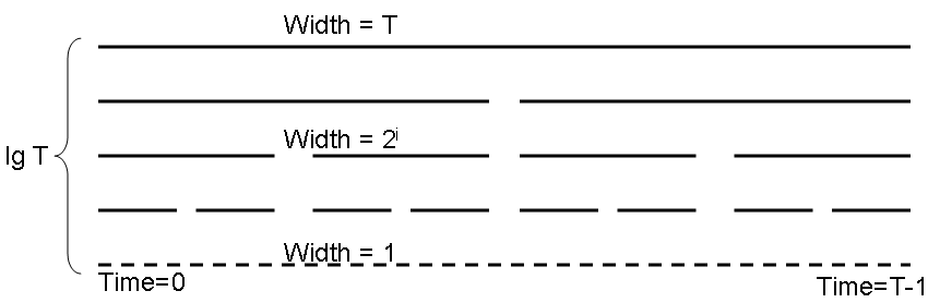
Specifically, we pre-compute the counts of all tags within a special set of intervals at various different scales. Figure 3 shows the intervals that are pre-computed. For simplicity, we assume T is a power of 2. As the figure shows, for each power of two, say 2i, with i=1,…,lg T, we cover all the days with intervals of length 2i and for each such interval we pre-compute a list of all objects that occur during the interval, sorted by interestingness. For example, at length scale 23=8, we pre-compute intervals [0,8], [8,16], [16,24], [24,32], …. Likewise for all powers of 2 between 1 and lg T. Because there are fewer and fewer intervals at each increasing length scale, the total storage for all these intervals only doubles the original data representation, and may reside on disk during processing. Further, we will later see that in practice, it is possible to store much less additional information -- details are in Section 5.
In order to perform a query for a particular interval I, we first express I as a combination of some of these pre-computed intervals, and then scan the data for all objects contained within each of the pre-computed intervals. Based on this information, we find the most interesting objects. We study two ways to combine pre-computed intervals: unions of intervals, and combinations of unions and set differences.
At run-time, we are given an interval [t,t+w] and the goal is to compute the top k most interesting objects in this interval. There are two steps to do this:
Our first algorithm, called Additive, has a decomposition step that expresses I as a disjoint union of pre-computed intervals, i.e., it computes a candidate set J such that I = ∪J ∈ J J. It has the advantage that it can make use of a provably optimal threshold algorithm [3] for the aggregation step. The second algorithm, termed subtractive, has a decomposition step that obtains a possibly more succinct decomposition by expressing I as both union and difference of pre-computed intervals, i.e., it obtains a candidate set J = J+ ∪ J- such that I = (∪J ∈ J+ J) \ (∪J ∈ J- J). However, the threshold algorithm is not directly applicable in this case and we have to modify it appropriately.
We illustrate the additive and subtractive decompositions with a concrete example. Suppose I=[0,63]. Then, the decomposition step of the additive algorithm will express it as I = [0, 32] ∪ [32, 48] ∪ [48, 56] ∪ [56, 60] ∪ [60, 62] ∪ [62, 63]. On the other hand, a more succinct expression of I is possible if we allow set differences: I = [0,64] \ [63, 64], which will in fact be the result of the decomposition step of the subtractive algorithm.
The algorithm for the decomposition step is as follows.
Interval Decomposition Algorithm (Additive).
Given an arbitrary interval [a,b], we identify the largest interval I'=[a',b'] in the pre-computed set that is completely contained in I, i.e., I' ⊆ I; this can be done very efficiently by examining b-a and a. We add this pre-computed interval to the collection, and then recurse on the subintervals [a,a'] and [b',b], as long as they are non-empty.
The following can be easily shown.
We now turn to the aggregation step. Recall that each pre-computed interval stores all objects that occur within the interval, ranked by interestingness within the interval. We must use this information as efficiently as possible to compute the most interesting objects within the query interval I. To do this, we employ the Threshold Algorithm (TA) of Fagin, Lotem, and Naor [3]. The algorithm is straightforward and we now describe it in its entirety.
The setting for Algorithm TA is as follows. We have a universe of objects, each of which has been scored on m separate dimensions. A function f combines the scores for each of the dimensions into a single overall score for the object. Our goal is to find the k objects with highest total score. For each dimension, a list of the objects is available sorted in order of score for that dimension. The score function f is assumed to be monotone: if one object scores at least as high as another in every dimension, it cannot be ranked lower overall. Some examples of monotone score functions are the sum of the scores, or the max of the scores, or a weighted combination of the scores. The goal now is find the objects with the highest aggregate scores according to f. Algorithm TA proceeds as follows:
Threshold Algorithm (Monotone).
Access in parallel each of the m sorted lists, in any order. For each element, look up its score in all m dimensions, and compute its overall score using f. Let xi be the score in the i-th dimension of the last object seen in the i-th list. Define τ = f(x1,…xm). Once k objects have been seen whose overall score is at least τ, terminate and return the k top objects seen so far.
Fagin et al. show that this algorithm is correct, and in fact is
optimal for aggregation in a strong sense they define.
Our interval covering problem falls directly into this framework. For a query interval I, we represent I as a union of intervals I1 ∪ … ∪ Il. For each object u, the score for each interval Ij is simply Int(u, Ij). Due to the linearity of Int, these scores may be combined by simple addition, which is a monotone combination of the scores from each interval. Thus, Algorithm TA may be applied to find the top k elements.
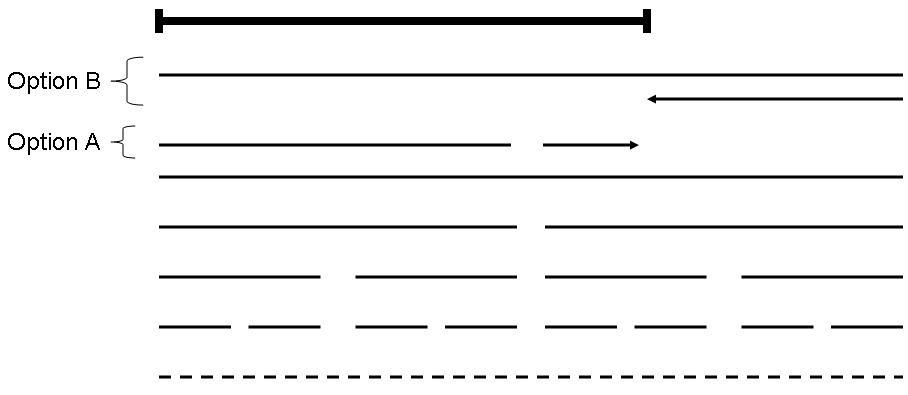
To obtain the decomposition using both additions (unions) and subtractions (set differences), we first consider a simpler problem: what if the query interval I is of the form [0,B]; that is, the left endpoint is zero. This case may be recast as the following problem: given an integer B, express it as sums and differences of powers of 2 in the shortest possible way. Figure 4 gives a graphical representation of this problem. The bold query interval in the figure may be covered using one of two options. In option A, we take the largest pre-computed interval contained entirely within I, and then recursively cover the remainder of I. In option B, we take the smallest pre-computed interval that completely covers I, and then recursively ``subtract off'' the remainder interval between I and the covering interval. The algorithm simply chooses the option that minimizes the length of the remainder interval. We may formally write this algorithm in terms of the right endpoint B as follows:
Integer Decomposition Algorithm (Subtractive).
Let ρ(I) denote the optimal representation of [0,I] using both addition and subtraction. Let b be the minimum number of bits needed to represent B. If B > 3 ⋅ 2b-2, then ρ(B) = [0, 2b] \ ρ(2b - B). If B ≤ 3 ⋅ 2b-2 then ρ(B) = [0, 2b-1] ∪ ρ(B-2b-1).
We can show the following by induction (proof omitted in this
version):
Thus, we can express every number B as ∑i pi - ∑i qi where pi's and qi's are powers of 2.
We now extend this result to provide an optimal algorithm for covering an arbitrary interval I using unions and set differences. The following shows that we may apply our algorithm for left-aligned intervals even if the interval is shifted by a sufficiently large power of 2, and the proof is immediate by a shifting argument:
In a straightforward manner, we may also extend to right-aligned intervals I = [2a - B, 2a], obtaining ρ(I) using ρ(B).
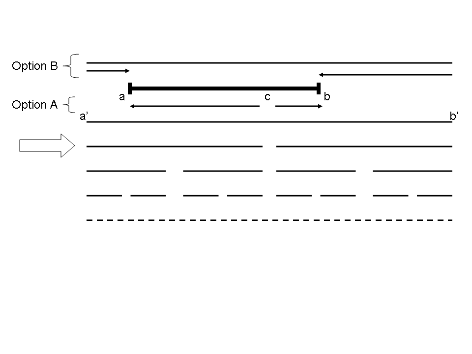
Now, we can construct an algorithm to decompose an arbitrary interval [a,b] into unions and set differences (additions and subtractions) of pre-computed intervals. The idea is given in Figure 5. As the figure shows, there are two options for representing I. We begin by identifying the smallest power of two such that no pre-computed interval of that width is contained in I. This width is indicated by the large block arrow on the left of the figure. I must cover the right endpoint of exactly one interval of this length -- let c be the location of that endpoint. Similarly, some pre-computed interval of twice that length must cover I; let J=[a',b'] be that interval. If x is the number of bits needed to represent the length of I, then note that a',b', and c are all multiples of powers of 2 greater than or equal to x2; we will use this fact later. We identify two options for optimally representing I. In option A, we consider covering I using the intervals [a,c] and [c,b], both of which are shifted left-aligned intervals by our earlier observation, and may therefore be covered optimally using our technique above. In option B, we begin by taking J, and then remove [a',a] and [b',b], both of which are also shifted left-aligned intervals and hence amenable to our earlier technique. We simply compare these two possible solutions, and report the best. The arrowheads in the figure show the direction in which the sub-intervals are aligned.
The following can be shown using a case analysis (proof omitted
here).
Notice that the aggregation function is given by the actual decomposition: if I = (∪J ∈ J+ J) \ (∪J ∈ J- J), then Int(u, I) = ∑J ∈ J+ Int(u, J) - ∑J ∈ J- Int(u, J). Therefore, the aggregation function f is no longer monotone and so we cannot use Algorithm TA.
However, notice that f is of a very special form: f=f+-f-, where f+,f- are monotone. Now we have two options to find the k objects with the highest f scores. There are two algorithms based on the kind of access model that is available. The first algorithm works when the only access available is to objects sorted by their f+ and f- scores. For instance, this is the case if we were to use TA to find the objects with highest/lowest f+ and f- scores. The second, more efficient algorithm works if, in addition to sorted access, we can random access the f+ or f- score of an object; this is inspired by TA.
Threshold Algorithm (Non-monotone, sorted access).
Access in parallel the objects ordered by f+ and those ordered by -f-. Continue until the same k objects appear in both lists. Output these k objects with top aggregated scores.
Threshold Algorithm (Non-monotone, random access).
Access in parallel the objects ordered by decreasing values of f+ and those ordered by increasing values of f-. As an object is seen under sorted access in one of the lists, do random access to the other list to find its score. For f+,f-, let x+,x- be the score of the last object seen under sorted access. Define the threshold value τ=x+-x-. As soon as at least k objects have been seen whose aggregate score is at least τ, stop. Finally, output the k objects with top aggregated scores.
It is easy to show:
It is also possible to obtain incremental versions of both the additive and subtractive algorithms. These algorithms take advantage of the fact that most of the time, the optimal representation for an interval [t,t+w] is related to the optimal representation for the next timestamp [t+1,t+1+w]. We omit the details of this algorithm in this version, and simply state the following proposition:
That is, as we slide an interval, the additive and subtractive algorithms produce a cover that changes on average by only a small (constant) number of members. Thus, if we count the number of pre-computed intervals that must be accessed to compute the most interesting objects at a particular query interval offset, the amortized cost of those accesses is small for each additional slide of the query interval.
<.<197>>
The data was obtained from Flickr (flickr.com), a Yahoo! property. Flickr is an extremely popular online photo-sharing site. Users can post photos on this site and annotate them with tags. Flickr also permits users to tag photos created by others.
The snapshot of Flickr data we analyzed had the following characteristics. The data consists of a table with the following columns: date, photo id, tagger id, and tag. There were 86.8M rows in this table, where each row represents an instance of a photo being tagged. Of these tags, around 1.26M were unique; thus each tag is repeated, on average, 70 times. The data spanned 472 days, starting June 3, 2004; thus, on average, more than 1.2M tags arrive per week.
First, we performed some simple data cleaning operations on this table. We extracted the raw tags and removed white space, punctuation, and converted them to lower case. This performs some simple normalization. We did not attempt to stem or spell-correct the tags since many of the tags were proper nouns (e.g., Katrina) or abbreviations (e.g., DILO, which means `Day In the Life Of').
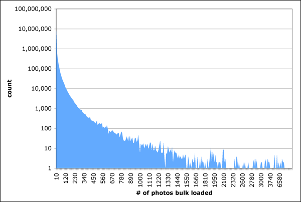
We used the `user id' field to ensure that on each day, a tag is counted only once per user, i.e., for a given user on a given day, we do not allow the user to place the same tag on different photos. This is to discount bulk uploads of many photos with same tag that might make these tags appear interesting for the wrong reason; in fact, as Figure 6 shows, this is a very common occurrence in Flickr. In other words, we implicitly want to capture the ``interestingness'' from a social perspective, and not an individual perspective. A global analysis of tag occurrences reveals the most commonly occurring tags are: 2005, 2004, and flowers. These tags, while very common, are unlikely to be particularly interesting for any reasonable interval in time. The `idf' term in our definition of interestingness guards against this: tags don't become interesting by virtue of occurring too often globally. As we mentioned earlier, the regularization parameter C in Equation 1 ensures that tags occur sufficiently many times globally before they can be considered interesting; we set C=50. We set k, the number of tags to display per interval, to be 8. We also compute their interestingness score for use in the visualization.
Our system consists of two parts. The back-end implements the algorithm described in Section 4 to find the most interesting 8 tags for every interval. This data is then written out to an intermediate data file. The front-end handles the visualization. The core component of the front-end is built using ActionScript and Flash MX. This portion consumes the data file and renders the tags on the screen, along with some sample photos for the tags, taken from the Flickr website.
In this section we discuss the performance of our back-end. Recall that the goal of our algorithm is to compute the most ``interesting'' tags during a particular interval of time. We will describe a naive scheme that uses no pre-processing, then a scheme that uses interval covering but no score aggregation, and finally our full scheme using both interval covering and score aggregation. We give performance numbers for all three approaches on various different interval widths.
Recall the Naive algorithm of Section 4 operates as follows: scan the data for each day contained in the query interval, and add up the interestingness scores for each tag. Report the top 8 scores. This approach uses no indexing whatsoever. We will refer to this scheme as ``Naive'' in the timing numbers below.
To perform interval covering, we first pre-compute the interestingness scores of all tags within the pre-computed intervals described in Section 4, as shown in Figure 3. In order to perform a query for a particular interval I, we first express I as a combination of pre-computed intervals, and then scan the tags associated with each of these pre-computed intervals, aggregating the interestingness scores. Based on this information, we find the eight most interesting tags, with their scores. We consider a much smaller number of intervals than in the Naive algorithm, but we still consider every tag occurring in each interval.
Our third scheme uses both interval covering and Algorithm TA. In this scheme, we again express the query interval in terms of pre-computed intervals. However, we do not examine every tag within each of the pre-computed intervals. Instead, we examine tags in order until we can conclude that no unseen tags could be more ``interesting'' than the tags we have seen so far, and we then terminate exploration.
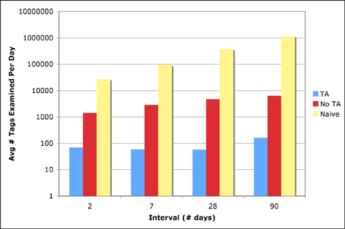
We examine performance for four different interval lengths: two days, one week, one month, and one quarter. For each interval length, we apply our backend to compute the most interesting tags for an interval of that length, at many different start locations, and take the average. We compare the naive algorithm (``Naive''), the additive interval covering algorithm without using the threshold algorithm (``No TA''), and the full additive interval covering algorithm with Algorithm TA (``TA''). As data access is the dominant factor in performance, Figure 7 shows the total number of tag interestingness scores that must be extracted in order to compute the eight most interesting tags. Thus, if a particular approach partitions the query [0,5] into [0,4] ∪ [4,5], and then scans 50 tags in the first interval, and 25 in the second, before concluding, then we charge this approach 75 accesses. All three algorithms return the optimal solution, but examine differing amounts of data. The y axis is plotted on a log scale in order to capture the differences. The naive algorithm examines between ten thousand and one million tag interestingness scores over the various different interval lengths. The ``No TA'' algorithm examines between one and two orders of magnitude fewer values: about one thousand values for length-2 intervals and almost ten thousand values for intervals of ninety days. Finally, the ``TA'' algorithm performs better yet, another one to two orders of magnitude improvement, examining around one hundred values for each interval. Thus, both the interval covering and the threshold algorithm provide a dramatic improvement over the naive algorithm, and the combination allows a highly efficient backend that can easily keep up with a browsing user.
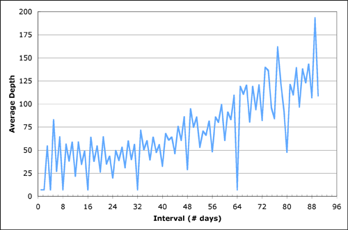
Recall that the threshold algorithm does not need to explore every tag during every pre-computed interval. Instead, it scans down the pre-computed intervals to a certain depth until it can determine that its solution is optimal. We may therefore examine how many tags it must explore per pre-computed interval before it is able to terminate. Figure 8 shows the average number of tags that must be explored per pre-computed intervals for a variety of interval lengths. The spikes at powers of two in the figure arise because these intervals may be expressed very succinctly in terms of pre-computed intervals -- the difference is quite dramatic because we perform experiments on an interval of width w at locations 0, w, 2w, …. The average depth ranges from around forty for short intervals to as much as two hundred for longer intervals. In all cases, these averages are quite small, explaining why the timing advantage is so significant.
However, this finding suggests another possible extension. If the algorithm explores only a prefix of the tags associated with each pre-computed interval, perhaps it is not necessary even to store the information for tags that will never be accessed. To evaluate this hypothesis, we compute the most tags ever extracted from any pre-computed interval during a series of runs of TA. We can then ask how many stored tags would be sufficient to provide optimal solutions for 99% of the queries, 95% of the queries, and so forth. The results are shown in Table 1. The table shows that we need to keep around more tags than the average, but not too many more: the average number of tags consumed for various intervals ranges from about thirty to almost two hundred, while the max number of tags consumed reaches 645 at 99% accuracy.
Table 1: Accuracy vs interval depth.
| Interval | .99 | .95 | .90 | .85 | .80 |
|---|---|---|---|---|---|
| 2 | 645 | 374 | 270 | 153 | 46 |
| 7 | 280 | 194 | 135 | 103 | 89 |
| 28 | 229 | 150 | 107 | 86 | 74 |
| 90 | 586 | 357 | 294 | 246 | 217 |
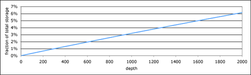
Armed with this information, we may then ask the benefit question: if we are willing to provide approximate answers in 1% of the cases, what storage savings will we discover? We perform the following experiment. Fix a cutoff d for the depth, and for each pre-computed interval, store only values for d tags. The total storage required for each value of d is shown in Figure 9 as a percentage of the storage required without any cutoff. Allowing 1% of queries to produce an approximate answer, as in our motivating question above, requires that we keep only 2% of the total storage.
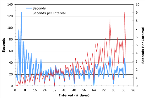
Finally, we can explore the actual timings for the TA algorithm, over interval widths ranging from two days to ninety days. Figure 10 shows the results. The thick line represents the total number of seconds
We now provide a few qualitative and anecdotal observations about the results of applying the algorithms described above. We begin by covering the types of tags that show up as ``interesting,'' and then move to a discussion of the impact of timescale.
Many of the ``interesting'' tags are quirky and unusual, and the reader is invited to explore them through the available demonstration system at http://research.yahoo.com/taglines. However, many fall into certain recurring categories, which we now describe.
There is significant bursty tagging behavior around special events. These include annually recurrent events such as holidays; for example, Valentine's Day, Thanksgiving, Xmas, and Hanukkah. However, they also include events on multi-year cycles such as Republican National Convention (Aug. 30, 2004), and a wide variety of one-off events. To give a sense of these events, here is a partial listing: Web_2.0 (Oct. 9), Lunar eclipse (Oct. 28), NYC Marathon (Nov. 8), GoogleFest (Aug. 23), Creepy Christmas (Dec 18), Flickr.Taiwan (Apr. 10), Googletalk (Aug. 24), Katrina Relief Auction (Sep. 1), Sith (May 20).
Photographs and tags tend to follow significant personalities in the news, particularly when those personalities exhibit strong temporal correlation. Examples include Jeanne Claude (Feb 18, 2005) and Pope (Apr. 26).
Certain interesting tags arise from the Flickr community itself, as users find interest in an apparently random topic and begin creating a body of tagged images around it. Examples include What's in your fridge? (Oct. 24-actual photos of the interior of refrigerators), Faces_in_holes (Nov. 21-faces visible through varieties of annuli), dilodec04 (Dec. 20-day in the life of), What's in your bag? (Mar. 10-images of the contents of people's bags), Badge (Jul. 1-images of access badges), Do your worst (Jul. 28-collection of the most unflattering photos), and White hands (Jul. 9-white hands!).
We alluded earlier to a qualitative difference in the types of tags that arise at a short timescale like a single day versus a longer timescale like one or more months. To wit, longer timescales tend to contain broader and more sustainable trends, while shorter scales tend to surface quirky and individualistic tags. Tags corresponding to regions of time such as july_2005 and AUGUST2005 occur only at larger timescales. At the three month timescale, tags such as INTERESTINGNESS and I LOVE NATURE begin to arise -- these have ``staying power'' with the users and have attracted something of a following.
In the other direction, tags that arise at the level of an individual day, but not a week or longer include short-duration activities such as LoveParadeSF and brief, quirky social activities like What's in your fridge.
At the day and week level, but not propagating to months or quarters, we see nycmarathon and Katrina Relief Auction. Then at the level of a month, but failing to reach the quarterly timescale, we see tags like lunar eclipse.
It is interesting to note that RNC Protest shows up only at the daily level, while the more general tag rnc shows up at all timescales.
We studied the problem of visualizing the evolution of tags within Flickr. We presented a novel approach based on a characterization of the most salient tags associated with a sliding interval of time. We developed an animation paradigm (using Flash) in a web browser, allowing the user to observe and interact with interesting tags as they evolve over time. In the course of this, we develop new algorithms and data structures to support an efficient generation of this visualization.
It will be interesting to extend this visualization to other online sources of data that have a temporal component, including news headlines, query logs, and music downloads.
We would like to thank the Flickr team for their help with data and discussions, particularly Serguei Mourachov, Stewart Butterfield, and Catarina Fake.
[1] J. Allan, J. Carbonell, G. Doddington, J. Yamron, and Y. Yang. Topic detection and tracking pilot study: Final report. DARPA Broadcast News Transcription and Understanding Workshop, 1998.
[2] S. Chien and N. Immorlica. Semantic similarities between search engine queries using temporal correlation. In Proceedings of the 14th International Conference on World Wide Web, pages 2-11, 2005.
[3] R. Fagin, A. Lotem, and M. Naor. Optimal aggregation algorithms for middleware. Journal of Computer and System Sciences, 66(4):614-656, 2003.
[4] S. Golder and B. Huberman. The structure of collaborative tagging systems. Journal of Information Science, 2006.
[5] A. Guttman. R-trees : A dynamic index structure for spatial searching. In Proceedings of the ACM SIGMOD International Conference on Management of Data, pages 47-57, 1984.
[6] M. Hadjieleftheriou, G. Kollios, V. J. Tsotras, and D. Gunopulos. Efficient indexing of spatiotemporal objects. In Proceedings of the 8th International Conferences on Extending Database Technology, pages 251-268, 2002.
[7] S. Havre, B. Hetzler, and L. Nowell. ThemeRiver: Visualizing thematic changes in large document collections. IEEE Transactions on Visualization and Computer Graphics, 8(1):9-20, 2002.
[8] J. Kleinberg. Bursty and hierarchical structure in streams. Data Mining and Knowledge Discovery, 7(4):373-397, 2003.
[9] J. Kleinberg. Temporal dynamics of on-line information systems. In M. Garofalakis, J. Gehrke, and R. Rastogi, editors, Data Stream Management: Processing High-Speed Data Streams. Springer, 2006.
[10] H. Korth and A. Silberschatz. Database System Concepts. McGraw-Hill, second edition, 1991.
[11] R. Kumar, J. Novak, P. Raghavan, and A. Tomkins. On the bursty evolution of blogspace. World Wide Web, 8(2):159-178, 2005.
[12] J. Lin, E. J. Keogh, S. Lonardi, J. P. Lankford, and D. M. Nystrom. Viztree: a tool for visually mining and monitoring massive time series databases. In Proceedings of International Conference on Very Large Data Bases, pages 1269-1272, 2004.
[13] B. Milash, C. Plaisant, and A. Rose. Lifelines: visualizing personal histories. In Proceedings of the International Conference Companion on Human Factors in Computing Systems, pages 392-393, 1996.
[14] D. Millen, J. Feinberg, and B. Kerr. Social bookmarking in the enterprise. ACM Queue, 3(9):28-35, 2005.
[15] S. Robertson and S. Walker. Okapi/Keenbow at Trec-8. In Proceedings of the 8th Text Retrieval Conference, pages 151-161, 2000.
[16] M. T. Roth, M. Arya, L. Haas, M. Carey, W. Cody, R. Fagin, P. Schwarz, J. Thomas, and E. Wimmers. The Garlic project. In Proceedings of the ACM SIGMOD International Conference on Management of Data, page 557, 1996.
[17] S. Saltenis, C. Jensen, S. Leutenegger, and M. A. Lopez. Indexing the positions of continuously moving objects. In Proceedings of the ACM SIGMOD International Conference on Management of Data, pages 331-342, 2000.
[18] B. Shneiderman. Tree visualization with tree-maps: 2-d space-filling approach. ACM Transactions on Graphics, 11(1):92-99, 1992.
[19] M. Vlachos, C. Meek, Z. Vagena, and D. Gunopulos. Identifying similarities, periodicities, and bursts for online search queries. In Proceedings of the ACM SIGMOD International Conference on Management of Data, pages 131-142, 2004.
[20] I. Witten, A. Moffat, and T. Bell. Managing Gigabytes. Morgan Kaufmann Publishers, second edition, 1999.
[21] Y. Yang, T. Pierce, and J. Carbonell. A study on retrospective and on-line event detection. In Proceedings of the 21st Annual International ACM Conference on Research and Development in Information Retrieval, pages 28-36, 1998.